B-Spline Foundation

Definition and Composition of B-Spline

Definition

A B-spline is a piecewise polynomial curve widely used in computer graphics, geometric modeling, and numerical analysis. It is composed of control points, a knot vector, and basis functions. Its mathematical expression is:

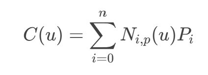
Where Pi are the control points, which define the shape of the curve; Ni,p(u) are the B-spline basis functions, which combine the control points with weights to form the curve; p is the degree of the B-spline, and u is the parameter, whose range is determined by the knot vector.

Composition

A B-spline consists of control points, a knot vector, basis functions, degree, and weights.

Control Points

Control points are the geometric definition points of the B-spline curve, determining its shape and direction.

Knot Vector

The knot vector is a non-decreasing sequence of real numbers U = {u0, u1, ..., um}, which defines the piecewise intervals of the parameter space. The knot vector can be uniform (equal spacing between the knots) or non-uniform (the spacing between the knots can vary). Knot multiplicity is also involved, which refers to the number of times a specific knot value appears in the knot vector. For example, in the knot vector {0, 0, 0, 1, 2, 2, 3}, the multiplicity of knot 0 is 3, the multiplicity of knot 1 is 1, the multiplicity of knot 2 is 2, and the multiplicity of knot 3 is 1.

Basis Function

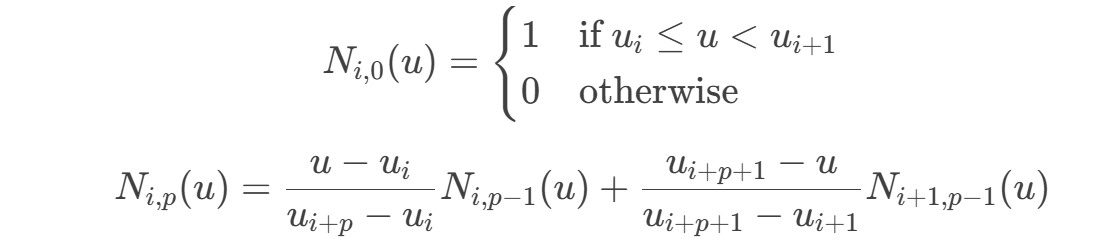
The B-spline basis function Ni,p(u) is calculated recursively:

The basis function determines the contribution of the control points to the shape of the curve.

Degree

The degree p is the polynomial degree of the B-spline. The higher the degree, the smoother the curve.

Weight

Standard B-spline do not have weights, and all control points have a default weight of 1. Rational B-spline (NURBS) introduce weights, allowing the representation of more complex geometries (such as conic curves). The weights can adjust the influence of control points on the shape of the curve.

Classification of B-Spline

B-spline can be classified based on different characteristics. Common classifications include uniform B-spline, non-uniform B-spline, periodic B-spline, non-periodic B-spline, and rational B-spline (NURBS). Below are their detailed descriptions:

Uniform B-Spline

Uniform B-spline have a knot vector that is evenly spaced along the parameter axis, i.e., ui+1 - ui = constant (>0). For example, the knot vector {0, 1, 2, 3, 4, 5, 6} has a uniform spacing of 1 between the knots.

Non-Uniform B-spline

Non-uniform B-spline have a knot vector that is non-uniformly distributed, i.e., the intervals between the knots may not be equal. The form of the knot vector can be any non-decreasing sequence, such as {0, 0.5, 1.2, 2.0, 3.5}.

Periodic B-spline

Periodic B-spline have a periodic knot vector, meaning the curve is continuous at both ends of the parameter domain. They are typically used to represent closed curves.It should be noted that for periodic B-spline curves, the multiplicities of the first and last knots in the knot vector must be equal. Additionally, tthe number of control points equals the sum of the knot multiplicities minus the multiplicity of the last knot For periodic B-splines, the condition ( m = n + p + 1 ) does not need to be satisfied.

std::vector< AMCAX::Point3 > pts2;
pts2.push_back(AMCAX::Point3(0., 0., 0.));
pts2.push_back(AMCAX::Point3(1., 1., 0.));
pts2.push_back(AMCAX::Point3(2., 2., 2.));
pts2.push_back(AMCAX::Point3(3., -5., 0.));
pts2.push_back(AMCAX::Point3(0., 0., 0.));
 
const std::vector< double > knots2 = { 0.,0.5, 1.,1.5, 2.0, 2.5};
const std::vector< int > multiplicities2 = { 1, 1, 1, 1, 1, 1};
 
int degree2 = 4;
std::shared_ptr< AMCAX::Geom3BSplineCurve> bspline2 = std::make_shared< AMCAX::Geom3BSplineCurve>(pts2, knots2, multiplicities2, degree2, true);
AMCAX::OCCTIO::OCCTTool::Write(AMCAX::MakeEdge(bspline2), "bspline2.brep");

In the example above, the multiplicities of the first and last knots in the knot vector are both 1. The number of control points equals the sum of the knot multiplicities minus the multiplicity of the last knot, which is 5 in both cases.

Non-Periodic B-spline

Non-periodic B-spline have a non-periodic knot vector, meaning the curve typically coincides with the first and last control points at the ends of the parameter domain. They are typically used to represent open curves.

std::vector< AMCAX::Point3 > pts1;
pts1.push_back(AMCAX::Point3(0.,0.,0.));
pts1.push_back(AMCAX::Point3(1.,1.,0.));
pts1.push_back(AMCAX::Point3(2.,2.,2.));
pts1.push_back(AMCAX::Point3(3.,-5.,0.));
const std::vector< double > knots1 = { 1.,2. };
const std::vector< int > multiplicities1 = { 4,4 };
int degree = 3;
std::shared_ptr< AMCAX::Geom3BSplineCurve> bspline1 = std::make_shared< AMCAX::Geom3BSplineCurve>(pts1, knots1, multiplicities1, degree, false);
AMCAX::OCCTIO::OCCTTool::Write(AMCAX::MakeEdge(bspline1), "bspline1.brep");

In the example above, the number of control points is 4, the degree of the curve is 3, the sum of the knot multiplicities is 8, and the total length of the knot vector satisfies ( m = n + p + 1 ).

Rational B-spline (NURBS)

Rational B-spline are an extension of B-spline, supporting more complex geometric shapes. NURBS introduce weights (positive numbers) to allow the representation of conic curves (e.g., circles, ellipses, parabolas), and the weights adjust the shape of the curve, making it more flexible.

std::vector<AMCAX::Point3> pts3 = {
AMCAX::Point3(0., 0., 0.),
AMCAX::Point3(1., 1., 0.),
AMCAX::Point3(2., 2., 2.),
AMCAX::Point3(3., -5., 0.)
};
 
std::vector<double> knots3 = {1., 2., 3., 4.};
std::vector<int> mults3 = { 2, 2, 2, 2};
std::vector<double> weights3 = { 1., 2., 1., 1.};
 
std::shared_ptr<AMCAX::Geom3BSplineCurve> bspline3 = std::make_shared<AMCAX::Geom3BSplineCurve>(pts3, weights3, knots3, mults3, 3, false, true);
AMCAX::OCCTIO::OCCTTool::Write(AMCAX::MakeEdge(bspline3), "bspline3.brep");
std::cout << bspline3->IsRational() << std::endl;//1

For a rational B-spline, the weights must be greater than 0 and not all equal. If all weights are equal, the rational B-spline will degenerate into a non-rational B-spline.

How to Construct a Valid B-Spline

To construct a valid B-spline, the following conditions must be met:

1.Control Points

• At least p+1 control points are needed. For example, for a 3rd-degree B-spline, at least 4 control points are required.

2.Knot Vector

• The total length of the knot vector must satisfy m=n+p+1, where n is the number of control points and p is the degree of the curve. (In the non-periodic case)
• The knot vector must be non-decreasing.

3.Knot Multiplicity

• For non-periodic B-splines, the multiplicities of the first and last knots in the knot vector must be equal, and the sum of the multiplicities after removing the last knot should be equal to the number of control points.
• The size of the knot multiplicity array must be equal to the size of the knot vector array.

Important Properties of B-spline

Tangency and Control Points at the Endpoints

For non-periodic B-spline, the tangent at the endpoints of the curve is aligned with the direction of the control points. For periodic B-spline, the tangency at the endpoints is usually not directly related to the control points, because the curve is closed. Below is an example of a non-periodic B-spline:

std::vector< AMCAX::Point3 > pts1;
pts1.push_back(AMCAX::Point3(0.,0.,0.));
pts1.push_back(AMCAX::Point3(1.,1.,0.));
pts1.push_back(AMCAX::Point3(2.,2.,2.));
pts1.push_back(AMCAX::Point3(3.,-5.,0.));
const std::vector< double > knots1 = { 1.,2. };
const std::vector< int > multiplicities1 = { 4,4 };
int degree = 3;
std::shared_ptr< AMCAX::Geom3BSplineCurve> bspline1 = std::make_shared< AMCAX::Geom3BSplineCurve>(pts1, knots1, multiplicities1, degree, false);
AMCAX::OCCTIO::OCCTTool::Write(AMCAX::MakeEdge(bspline1), "bspline1.brep");
 
double fp = bspline1->FirstParameter();
AMCAX::Point3 fpoint;
AMCAX::Vector3 fv;
bspline1->D1(fp, fpoint,fv);
std::cout << "First parameter: " << fp << std::endl;
std::cout << "Start point: " << fpoint << std::endl;
std::cout << "Start tangent: " << fv << std::endl;
 
AMCAX::Vector3 direction(
    pts1[1].X() - pts1[0].X(),
    pts1[1].Y() - pts1[0].Y(),
    pts1[1].Z() - pts1[0].Z()
);
std::cout << direction << std::endl;
 
if (fv.Normalized().IsEqual(direction.Normalized(), AMCAX::Precision::Confusion(), AMCAX::Precision::Angular()))
{
    std::cout << "The start tangent is consistent with the control point direction" << std::endl;
}
else {
    std::cout << "The start tangent is not consistent with the control point direction" << std::endl;
}

The Effect of Knot Multiplicity on Continuity

Knot multiplicity directly affects the continuity of the curve. The higher the multiplicity of a knot, the lower the continuity at that point. If a knot has multiplicity 1, the curve is C(p-1) continuous at that knot. If the multiplicity is k, the curve is C(p-k) continuous at that knot. If the multiplicity is p+1, the curve is discontinuous at that knot.

For a 3rd-degree B-spline (p=3):

• Multiplicity 1: The curve is C2 continuous at that knot.
• Multiplicity 2: The curve is C1 continuous at that knot.
• Multiplicity 3: The curve is C0 continuous at that knot.
• Multiplicity 4: The curve is discontinuous at that knot.

Affine Invariance

B-spline possess affine invariance, meaning that if affine transformations (such as translation, rotation, or scaling) are applied to the control points, the shape of the curve will change accordingly, but the parametric form of the curve remains unchanged. This implies that the relative structure and shape of the B-spline curve are always preserved, regardless of how affine transformations are applied to the control points.